Software for design optimization: Difference between revisions
| Line 124: | Line 124: | ||
=== How does the DTC Toolkit calculate resolution? === | === How does the DTC Toolkit calculate resolution? === | ||
The resolution in this case is defined as the width of the final range histogram for all protons. | The resolution in this case is defined as the width of the final range histogram for all protons. | ||
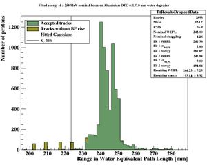
The goal is to match the range straggling which manifests itself in the Gaussian distribution of the range of all protons in the DTC, from the full Monte Carlo simulations: | |||
[[File:findRanges_onlyrange.JPG|300px]] | |||
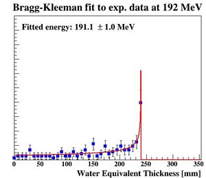
To characterize the resolution, a realistic analysis is performed. Instead of scoring the complete detector volume, including the massive energy absorbers, only the sensor chips placed at intervals (<math>\Delta z = 0.375\ \textrm{mm} + d_{\textrm{absorber}}</math>) are scored. Tracks are compiled by using the eventID tag from GATE, so that the track reconstruction efficiency is 100%. Each track is then put in a depth / edep graph, and a Bragg curve is fitted on the data: | |||
[[File:BK fit.JPG|300px]] | |||
The distribution of all fitted ranges (simple to calculate from fitted energy) should match the distribution above - with a perfect system. All degradations during analysis, sampling error, sparse sampling, mis-fitting etc. will ensure that the peak is broadened. | |||
[[File:distribution_after_analysis.JPG|300px]] | |||
=== Finding the resolution === | === Finding the resolution === | ||
Revision as of 20:45, 27 February 2017
Required software
In order to run the software to generate the geomtry, Monte Carlo data and do full simulations, you need the following software:
- ROOT
- Geant4
- Gate
- DTC toolkit (Helge's code)
GATE Simulations
Generating the geometry
To generate the geometry files to run in Gate, a Python script is supplied. It is located within the gate/python subfolder.
[gate/python] $ python gate/python/makeGeometryDTC.py
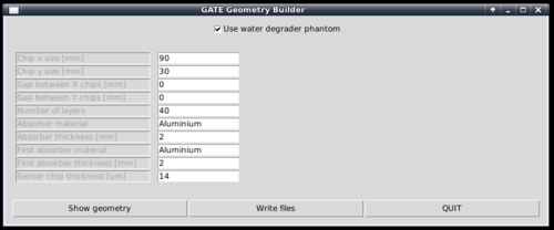
Choose the wanted characteristics of the detector, and use write files in order to create the geometry file Module.mac, which is automatically included in Main.mac
Creating the full simulations files for a range-energy look-up-table
First, enable the full scoring of all volumes by commenting / uncommenting in Main.mac:
   #/control/execute readout.mac
   /control/execute readout_full.mac
Then, in the same file, save to the correct ROOT file:
   /gate/output/root/setFileName ../../DTCToolkit/Data/MonteCarlo/DTC_Full_Aluminium_Absorber{absorberthickness}mm_Degrader{degraderthickness}mm_{energy}MeV
   #/gate/output/root/setFileName ../../DTCToolkit/Data/MonteCarlo/DTC_Aluminium_Absorber{absorberthickness}mm_{energy}MeV
It is not critical to have a high number of primaries in this part. 10000 is enough for this step. Change this in the Main.mac file! To loop through different energy degrader thicknesses, run the script runDegrader.sh:
[gate/python] $ sh runDegrader.sh <absorber thickness> <degraderthickness from> <degraderthickness stepsize> <degraderthickness to>
The brackets indicate the folder in the Github repository to run the code from. For example, with a 3 mm degrader, and simulating a 250 MeV beam passing through a phantom of 50, 55, 60, 65 and 70 mm water:
[gate/python] $ sh runDegrader.sh 3 50 5 70
Creating the chip-readout simulations files for resolution calculation
First, undo the changes to Main.mac:
   /control/execute readout.mac
   #/control/execute readout_full.mac
Then, in the same file, save to the correct ROOT file:
   #/gate/output/root/setFileName ../../DTCToolkit/Data/MonteCarlo/DTC_Full_Aluminium_Absorber{absorberthickness}mm_Degrader{degraderthickness}mm_{energy}MeV
   /gate/output/root/setFileName ../../DTCToolkit/Data/MonteCarlo/DTC_Aluminium_Absorber{absorberthickness}mm_{energy}MeV
In this step a higher number of particles is desired. I usually use 25000 since we need O(100) simulations. A sub 1-mm step size will really tell us if we manage to detect such small changes in a beam energy.
And loop through the different absorber thicknesses:
[gate/python] $ sh runDegrader.sh <absorber thickness> <degraderthickness from> <degraderthickness stepsize> <degraderthickness to>
Creating the basis for range-energy calculations
The range-energy look-up-table
Now we have ROOT output files from Gate, all degraded differently through a varying water phantom and therefore stopping at different places in the DTC. We want to follow all the tracks to see where they end, and make a histogram over their stopping positions. This is of course performed from a looped script, but to give a small recipe:
- Retrieve the first interaction of the first particle. Note its event ID (history number) and edep (energy loss for that particular interaction)
- Repeat until the particle is outside the phantom. This can be found from the volume ID or the z position (the first interaction with {math|z>0}). Sum all the found edep values, and this is the energy loss inside the phantom. Now we have the "initial" energy of the proton before it hits the DTC
- Follow the particle, noting its z position. When the event ID changes, the next particle is followed, and save the last z position of where the proton stopped in a histogram
- Do a Gaussian fit of the histogram after all the particles have been followed. The mean value is the range of the beam with that particular "initial" energy. The spread is the range straggling. Note that the range straggling is more or less constant, but the contributions to the range straggling from the phantom and DTC, respectively, are varying linearly.
This recipe has been implemented in DTCToolkit/Scripts/findRange.C. Test run the code on a few of the cases (smallest and biggest phantom size ++) to see that
- The correct start- and end points of the histogram looks sane. If not, this can be corrected for by looking how
xfromandxtois calculated and playing with the calculation. - The mean value and straggling is calculated correctly
- The energy loss is calculated correctly
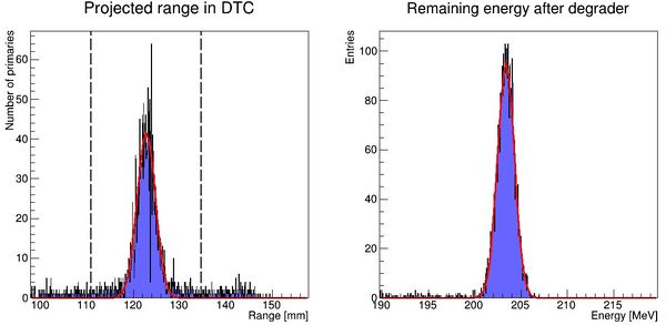
The output should look like this: Correctly places Gaussian fits is a good sign.
If you're happy with this, then a new script will run findRange.C on all the different ROOT files generated earlier.
   [DTCToolkit/Scripts] $ root
   ROOT [1] .L findManyRangesDegrader.C
   // void findManyRanges(Int_t degraderFrom, Int_t degraderIncrement, Int_t degraderTo, Int_t absorberThicknessMmFrom, Int_t absorberThicknessMmIncrement, Int_t absorberThicknessMmTo)
   ROOT [2] findManyRanges(50, 5, 70, 3, 1, 3)
The output is stored in DTCToolkit/Output/findManyRangesDegrader.csv.
It is a good idea to look through this file, to check that the values are not very jumpy (Gaussian fits gone wrong).
We need the initial energy and range in ascending order. The findManyRangesDegrader.csv files contains more rows such as initial energy straggling and range straggling for other calcualations. This is sadly a bit tricky, but do (assuming a 3 mm absorber geometry):
[DTCToolkit] $ cat OutputFiles/findManyRangesDegrader.csv | cut -d ' ' -f6,3 | awk '{print ($2 " " $1)}' Data/Ranges/3mm_Al.csv | sort -n > Data/Ranges/3mm_Al.csv
When this is performed, the range-energy table for that particular geometry has been created, and is ready to use in the analysis. Note that since the calculation is based on cubic spline interpolations, it cannot extrapolate -- so have a larger span in the full Monte Carlo simulation data than with the chip readout. For more information about that process, see this document: File:Comparison of different calculation methods of proton ranges.pdf
Range straggling parameterization and [math]\displaystyle{ R_0 = \alpha E^p }[/math]
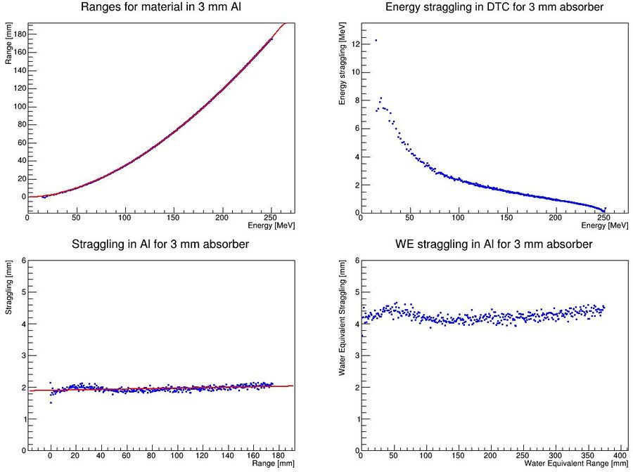
It is important to know the amount of range straggling in the detector, and the amount of energy straggling after the degrader. In addition, to calculate the parameters [math]\displaystyle{ \alpha, p }[/math] from the somewhat inaccurate Bragg-Kleeman equation [math]\displaystyle{ R_0 = \alpha E ^ p }[/math], in order to correctly model the "depth-dose curve" [math]\displaystyle{ dE / dz = p^{-1} \alpha^{-1/p} (R_0 - z)^{1/p-1} }[/math]. This is done by fitting the Bragg-Kleeman equation to the range-energy look up tables found by using DTCToolkit/Scripts/findManyRangesDegrader.C.
To find all this, run the script DTCToolkit/Scripts/findAPAndStraggling.C. This script will loop through all available data lines in the DTCToolkit/OutputFiles/findManyRangesDegrader.csv file that has the correct absorber thickness, so you need to clean the file first (or just delete it before running findManyRangesDegrader.C).
  [DTCToolkit/Scripts] $ root
  ROOT [0] .L findAPAndStraggling.C+
  // void findAPAndStraggling(int absorberthickness)
  ROOT [1] findAPAndStraggling(3)
The output from this function should be something like this:
In addition, the following parameters should be extracted:
   Bragg-Kleeman parameters: R = 0.011626 E ^ 1.743151
   Straggling = 1.8568 + 0.000856 R
   WE Straggling = 4.14806 + 0.000223 R
Running the DTC Toolkit
Configuring the DTC Toolkit to run with correct geometry
The values from findManyRanges.C should already be in DTCToolkit/Data/Ranges/3mm_Al.csv (or the corresponding material / thickness). Check that the file is correctly loaded in the file DTCToolkit/GlobalConstants/MaterialConstants.C. The values from findAPAndStraggling.C are put into the same file DTCToolkit/GlobalConstants/MaterialConstants.C:
   81  void createSplines() {
   ...
   107    else if (kAbsorbatorThickness = 3) {
   108       in.open("Data/Ranges/3mm_Al.csv");
   109    }
   ...
   192    else if (kAbsorbatorThickness = 3) {
   193       alpha_aluminum = 0.011626;
   194       p_aluminum = 1.743151;
   195       straggling_a = 1.8568;
   196       straggling_b = 0.000856;
   197    }
Or in the corresponding material (alpha_pmma, alpha_carbon, etc.) and absorbatorthickness lines.
Then, look in the file DTCToolkit/GlobalConstants/Constants.h and check that the correct absorber thickness values etc. are set:
  ...
  39 Bool_t useDegrader = true;
  ...
  52 const Float_t kAbsorberThickness = 3;
  ...
  59 Int_t kEventsPerRun = 100000;
  ...
  66 const Int_t kMaterial = kAluminum;
Since we don't use tracking but only MC truth in the optimization, the number kEventsPerRun ([math]\displaystyle{ n_p }[/math] in the NIMA article) should be higher than the number of primaries per energy.
How does the DTC Toolkit calculate resolution?
The resolution in this case is defined as the width of the final range histogram for all protons. The goal is to match the range straggling which manifests itself in the Gaussian distribution of the range of all protons in the DTC, from the full Monte Carlo simulations:
To characterize the resolution, a realistic analysis is performed. Instead of scoring the complete detector volume, including the massive energy absorbers, only the sensor chips placed at intervals ([math]\displaystyle{ \Delta z = 0.375\ \textrm{mm} + d_{\textrm{absorber}} }[/math]) are scored. Tracks are compiled by using the eventID tag from GATE, so that the track reconstruction efficiency is 100%. Each track is then put in a depth / edep graph, and a Bragg curve is fitted on the data:
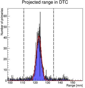
The distribution of all fitted ranges (simple to calculate from fitted energy) should match the distribution above - with a perfect system. All degradations during analysis, sampling error, sparse sampling, mis-fitting etc. will ensure that the peak is broadened.
