Software for design optimization

Required software

In order to run the software to generate the geomtry, Monte Carlo data and do full simulations, you need the following software:

ROOT
Geant4
Gate
DTC toolkit (Helge's code)

GATE Simulations

Generating the geometry

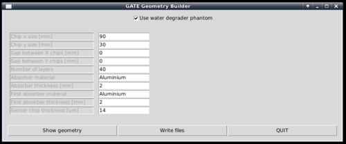
To generate the geometry files to run in Gate, a Python script is supplied. It is located within the gate/python subfolder.

   [gate/python] $ python gate/python/makeGeometryDTC.py

Choose the wanted characteristics of the detector, and use write files in order to create the geometry file Module.mac, which is automatically included in Main.mac

Creating the full simulations files for a range-energy look-up-table

First, enable the full scoring of all volumes by commenting / uncommenting in Main.mac:

   #/control/execute readout.mac
   /control/execute readout_full.mac

Then, in the same file, save to the correct ROOT file:

   /gate/output/root/setFileName ../../DTCToolkit/Data/MonteCarlo/DTC_Full_Aluminium_Absorber{absorberthickness}mm_Degrader{degraderthickness}mm_{energy}MeV
   #/gate/output/root/setFileName ../../DTCToolkit/Data/MonteCarlo/DTC_Aluminium_Absorber{absorberthickness}mm_{energy}MeV

It is not critical to have a high number of primaries in this part. 10000 is enough for this step. Change this in the Main.mac file! To loop through different energy degrader thicknesses, run the script runDegrader.sh:

   [gate/python] $ sh runDegrader.sh <absorber thickness> <degraderthickness from> <degraderthickness stepsize> <degraderthickness to>

The brackets indicate the folder in the Github repository to run the code from. For example, with a 3 mm degrader, and simulating a 250 MeV beam passing through a phantom of 50, 55, 60, 65 and 70 mm water:

   [gate/python] $ sh runDegrader.sh 3 50 5 70

Creating the chip-readout simulations files for resolution calculation

First, undo the changes to Main.mac:

   /control/execute readout.mac
   #/control/execute readout_full.mac

Then, in the same file, save to the correct ROOT file:

   #/gate/output/root/setFileName ../../DTCToolkit/Data/MonteCarlo/DTC_Full_Aluminium_Absorber{absorberthickness}mm_Degrader{degraderthickness}mm_{energy}MeV
   /gate/output/root/setFileName ../../DTCToolkit/Data/MonteCarlo/DTC_Aluminium_Absorber{absorberthickness}mm_{energy}MeV

In this step a higher number of particles is desired. I usually use 25000 since we need O(100) simulations. A sub 1-mm step size will really tell us if we manage to detect such small changes in a beam energy.

And loop through the different absorber thicknesses:

   [gate/python] $ sh runDegrader.sh <absorber thickness> <degraderthickness from> <degraderthickness stepsize> <degraderthickness to>

Creating the range-energy look-up-table

Now we have ROOT output files from Gate, all degraded differently through a varying water phantom and therefore stopping at different places in the DTC. We want to follow all the tracks to see where they end, and make a histogram over their stopping positions. This is of course performed from a looped script, but to give a small recipe:

Retrieve the first interaction of the first particle. Note its event ID (history number) and edep (energy loss for that particular interaction)
Repeat until the particle is outside the phantom. This can be found from the volume ID or the z position (the first interaction with {math|z>0}). Sum all the found edep values, and this is the energy loss inside the phantom. Now we have the "initial" energy of the proton before it hits the DTC
Follow the particle, noting its z position. When the event ID changes, the next particle is followed, and save the last z position of where the proton stopped in a histogram
Do a Gaussian fit of the histogram after all the particles have been followed. The mean value is the range of the beam with that particular "initial" energy. The spread is the range straggling. Note that the range straggling is more or less constant, but the contributions to the range straggling from the phantom and DTC, respectively, are varying linearly.

This recipe has been implemented in DTCToolkit/Scripts/findRange.C. Test run the code on a few of the cases (smallest and biggest phantom size ++) to see that

The correct start- and end points of the histogram looks sane. If not, this can be corrected for by looking how xfrom and xto is calculated and playing with the calculation.
The mean value and straggling is calculated correctly
The energy loss is calculated correctly

If you're happy with this, then a new script will run findRange.C on all the different ROOT files generated earlier.

   [DTCToolkit/Scripts] $ root 
   ROOT [1] .L findManyRangesDegrader.C
   // void findManyRanges(Int_t degraderFrom, Int_t degraderIncrement, Int_t degraderTo, Int_t mmFrom, Int_t mmIncrement, Int_t mmTo)
   ROOT [2] findManyRanges(50, 5, 70, 3, 1, 3)

The output is stored in DTCToolkit/Output/findManyRangesDegrader.csv.

We need the initial energy and range in ascending order. The findManyRangesDegrader.csv files contains more rows such as initial energy straggling and range straggling for other calcualations. This is sadly a bit tricky, but do (assuming a 3 mm absorber geometry):

  [DTCToolkit] $ cat OutputFiles/findManyRangesDegrader.csv | cut -d ' ' -f6,3 > Data/Ranges/3mm_Al.csv
  [DTCToolkit] $ awk '{print ($2 " " $1)}' Data/Ranges/3mm_Al.csv | sort -n > Data/Ranges/3mm_Al.csv

When this is performed, the range-energy table for that particular geometry has been created, and is ready to use in the analysis. Note that since the calculation is based on cubic spline interpolations, it cannot extrapolate -- so have a larger span in the full Monte Carlo simulation data than with the chip readout.