Software tutorial at IFT

Introduction and overview

This page is meant as a recipe for the software day at IFT, March 20 2017. We have decided that this should take place on Monday, March 20 between 09.00 am and 3.00 pm at the Department of Physics and Technology (our usual meeting room in the 5th floor).

There are certain steps you need to take prior to the meeting. We do not wish to loose time on installation and configuration of the software needed. Thus, it is imperative that you come with your laptops which already have the following installed and configured properly:

1. ROOT installation
2. Geant 4 installation
3. Gate installation
4. DTC Toolkit for reconstruction

Agenda for the day is as follows:

1. An introduction to GATE macros, i.e. GATE input scripts
2. Setting up a simple simulation geometry in GATE using a proton bencil beam and a water phantom
3. Running short simulations
4. Examination of the GATE-output files

We think that the above mentioned mini introduction to GATE should take no longer than 1 – 1.5 hours. Rest of the day, we will focus on a more in-depth review of the analysis code written by Helge P.

1. Setting up a tracking calorimeter geometry in GATE
2. Running short simulations with the detector geometry
3. Using the results of the MC simulations, a short «hands-on» introduction to Helge P.’s analysis code written in the Root framework
4. A review of all the different modules in the above mentioned analysis code

The final goals of the day will be:

1. Setting up a GATE simulation of an example tracking calorimeter including geometry, material specifications and proton beam definition
2. Being able to work with the GATE output files (identifying primary protons, secondary particles, calculating deposited dose etc…)
3. Being able to run a complete analysis using the Root-analysis code written by Helge P.

As always, check the User guide and tutorial for the DTC Toolkit to find a Wiki-friendly guide.

GATE

Simulations of Preclinical and Clinical Scans in Emission Tomography, Transmission Tomography and Radiation Therapy

Geant4 is a C++ library, where an application / simulation is built by writing certain C++ classes (geometry, beam, scoring, output, physics), and compiling the binaries from where the simulations are run. Only certain modifications to the simulations can be made with the binaries, such as beam settings, certain physics settings as well as geometry objects pre-defined to be variable.

GATE is an application written for Geant4. It was originally meant for PET and SPECT uses, however it is very flexible so many different kinds of detectors can be designed. To run GATE, only macro files written in the Geant4 scripting language (with some GATE specific commands) are needed to build the geometry, scoring, physics and beam. The output is also defined in the macro files, either to ASCII files or to ROOT files.

In each simulation, the user has to:

1. define the scanner geometry
2. set up the physics processes
3. initialize the simulation
4. set up the detector model
5. define the source(s)
6. specify the data output format
7. start the acquisition

Introduction to GATE macros

Gate, just as GEANT4, is a program in which the user interface is based on scripts. To perform actions, the user must either enter commands in interactive mode, or build up macro files containing an ordered collection of commands.

Each command performs a particular function, and may require one or more parameters. The Gate commands are organized following a tree structure, with respect to the function they represent. For example, all geometry-control commands start with geometry, and they will all be found under the /geometry/ branch of the tree structure.

When Gate is run, the Idle> prompt appears. At this stage the command interpreter is active; i.e. all the Gate commands entered will be interpreted and processed on-line. All functions in Gate can be accessed to using command lines. The geometry of the system, the description of the radioactive source(s), the physical interactions considered, etc., can be parameterized using command lines, which are translated to the Gate kernel by the command interpreter. In this way, the simulation is defined one step at a time, and the actual construction of the geometry and definition of the simulation can be seen on-line. If the effect is not as expected, the user can decide to re-adjust the desired parameter by re-entering the appropriate command on-line. Although entering commands step by step can be useful when the user is experimenting with the software or when he/she is not sure how to construct the geometry, there remains a need for storing the set of commands that led to a successful simulation.

Macros are ASCII files (with '.mac' extension) in which each line contains a command or a comment. Commands are GEANT4 or Gate scripted commands; comments start with the character ' #'. Macros can be executed from within the command interpreter in Gate, or by passing it as a command-line parameter to Gate, or by calling it from another macro. A macro or set of macros must include all commands describing the different components of a simulation in the right order. Usually these components are visualization, definitions of volumes (geometry), systems, digitizer, physics, initialization, source, output and start. These steps are described in the next sections. A single simulation may be split into several macros, for instance one for the geometry, one for the physics, etc. Usually, there is a master macro which calls the more specific macros. Splitting macros allows the user to re-use one or more of these macros in several other simulations, and/or to organize the set of all commands. To execute a macro (mymacro.mac in this example) from the Linux prompt, just type :

Gate mymacro.mac 

To execute a macro from inside the Gate environment, type after the "Idle>" prompt:

Idle>/control/execute mymacro.mac 

And finally, to execute a macro from inside another macro, simply write in the master macro:

/control/execute mymacro.mac 

Setting up a simple simulation geometry in GATE using a pencil beam and a water phantom

Visualization

First we may want to set up a visualization engine to see what's going on. This is optional, and runs in batch mode should not be visualized! Here we use the opengl visualizer OGLX, but different kinds of visualization engines are discussed in the GATE Wiki [[1]]

  /vis/open OGLSX
  /vis/viewer/reset
  /vis/viewer/set/viewpointThetaPhi 60 60
  /vis/viewer/zoom 1
  /vis/viewer/set/style surface
  /vis/drawVolume
  /tracking/storeTrajectory 1
  /vis/scene/endOfEventAction accumulate
  /vis/viewer/update

Most of these commands are self explainatory. By using the storeTrajectory command, all particles are displayed together with the geometry.

Materials database

The default material assigned to a new volume is Air. The list of available materials is defined in the GateMaterials.db file. It's included in the Gate folder, and should be copied to the active directory. It is easy to add new materials to the file, just have a look at the file.

  /gate/geometry/setMaterialDatabase MyMaterialDatabase.db

Geometry

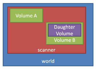
Apart from specialized geometries such as PET, SPECT, CT, the general geometry is called as scanner. It must be placed within the world volume, and all parts of the detector (to be scored) be placed within the scanner volume.

To construct a simple water phantom geometry of 30x30x30 cm, use the following commands:

  /gate/world/geometry/setXLength 1000. cm
  /gate/world/geometry/setYLength 1000. cm
  /gate/world/geometry/setZLength 1000. cm

So we've defined a world geometry of 1 m³. It must be larger than all its daughter volumes. Let's put the scanner volume inside the world volume. Since it's not already defined (the world volume was), we must insert a box object (with parameters XLength, YLength, ZLength as the side measurements of the box):

  /gate/world/daughters/name scanner
  /gate/world/daughters/insert box
  /gate/scanner/geometry/setXLength 100. cm
  /gate/scanner/geometry/setYLength 100. cm
  /gate/scanner/geometry/setZLength 100. cm
  /gate/scanner/placement/setTranslation 0 0 50. cm
  /gate/scanner/vis/forceWireframe

Inside this scanner volume (the default material is Air):

  /gate/scanner/daughters/name phantom
  /gate/scanner/daughters/insert box
  /gate/phantom/geometry/setXLength 30. cm
  /gate/phantom/geometry/setYLength 30. cm
  /gate/phantom/geometry/setZLength 30. cm
  /gate/phantom/placement/setTranslation 0 0 -15. cm
  /gate/phantom/setMaterial Water
  /gate/phantom/vis/forceWireframe

It is possible to repeat volumes. The simple method is to use a linear replicator:

  /gate/phantom/repeaters/insert linear
  /gate/phantom/linear/autoCenter false
  /gate/phantom/linear/setRepeatNumber 10
  /gate/phantom/linear/setRepeatVector 0 0 35. cm

The autoCenter command: The original volume is anchored (false), instead of the center-of-mass of all copies being centered at that position (true).

Sensitive Detectors

The scoring system in Geant4/GATE is based around Sensitive Detectors (SD). If a volume is a daughter volume (or granddaughter, ...), it may be assigned as a SD. This process is super simple in GATE:

  /gate/phantom/attachCrystalSD

If you want to define hierarchically repeated structures, such as layers or individually simulated pixels, they should be defined as a level:

  /gate/scanner/level1/attach phantom
  /gate/scanner/level2/attach repeatedStructureWithinPhantom

And now you can use the ROOT leaf level1ID and level2ID to identify the volume.

Physics

There are many physics lists to choose from in Geant4/GATE. For proton therapy and detector simulations, I most often use a combination of a low-energy-friendly hadronic list and the variable-steplength (for Bragg Peak accuracy) electromagnetic list. From the Geant4 reference physics webpage [[2]]:

• QGSP: QGSP is the basic physics list applying the quark gluon string model for high energy interactions of protons, neutrons, pions, and Kaons and nuclei. The high energy interaction creates an exited nucleus, which is passed to the precompound model modeling the nuclear de-excitation.
• QGSP_BIC: Like QGSP, but using Geant4 Binary cascade for primary protons and neutrons with energies below ~10GeV, thus replacing the use of the LEP model for protons and neutrons In comparison to the LEP model, Binary cascade better describes production of secondary particles produced in interactions of protons and neutrons with nuclei.
• emstandard_opt3 designed for any applications required higher accuracy of electrons, hadrons and ion tracking without magnetic field. It is used in extended electromagnetic examples and in the QGSP_BIC_EMY reference Physics List. The corresponding physics

The physics list to use all of these is called QGSP_BIC_EMY. It is loaded with the command

  /gate/physics/addPhysicsList QGSP_BIC_EMY

In addition, in order to accurately represent the water in the water phantom, we define the current recommended value for the mean ionization potential for water, which is [math]\displaystyle{ 75\ \mathrm{eV} }[/math]. This can be performed for all materials, and it will override Bragg's additivity rule.

  /gate/geometry/setIonisationPotential Water 75 eV

Initialization

After the geometry and physics has been set, initialize the run!

  /gate/run/initialize

Proton beam

  /gate/source/addSource PBS PencilBeam
  /gate/source/PBS/setParticleType proton
  /gate/source/PBS/setEnergy 188.0 MeV
  /gate/source/PBS/setSigmaEnergy 1.0 MeV
  /gate/source/PBS/setPosition 0 0 -10. mm
  /gate/source/PBS/setSigmaX 2 mm
  /gate/source/PBS/setSigmaY 4 mm
  /gate/source/PBS/setSigmaTheta 3.3 mrad
  /gate/source/PBS/setSigmaPhi 3.8 mrad
  /gate/source/PBS/setEllipseXThetaEmittance 15 mm*mrad
  /gate/source/PBS/setEllipseXThetaRotationNorm negative
  /gate/source/PBS/setEllipseYPhiEmittance 20 mm*mrad
  /gate/source/PBS/setEllipseYPhiRotationNorm negative
  /gate/application/setTotalNumberOfPrimaries 5000

It is tricky to use this beam since all parameters need to match, so an alternative is to use a uniform General Particle Source:

  /gate/source/addSource uniformBeam gps
  /gate/source/uniformBeam/gps/particle proton
  /gate/source/uniformBeam/gps/ene/type Gauss
  /gate/source/uniformBeam/gps/ene/mono 188 MeV
  /gate/source/uniformBeam/gps/ene/sigma 1 MeV
  /gate/source/uniformBeam/gps/type Plane
  /gate/source/uniformBeam/gps/shape Square
  /gate/source/uniformBeam/gps/direction 0 0 1
  /gate/source/uniformBeam/gps/halfx 0 mm
  /gate/source/uniformBeam/gps/halfy 0 mm
  /gate/source/uniformBeam/gps/centre 0 0 -1 cm
  /gate/application/setTotalNumberOfPrimaries 5000

Output

For this tutorial, we will use the ROOT output.

  /gate/output/root/enable
  /gate/output/root/setFileName gate_simulation

Running the simulation

To finalize the macro file, start the randomization engine and run!

  /gate/random/setEngineName MersenneTwister
  /gate/random/setEngineSeed auto
  /gate/application/start

Running short simulations

To run a simulation, create a macro file with the lines as descibed above, and run it with

  $ Gate waterphantom.mac

The terminal output describes the geometry, physics, etc. If you want the visualization to be persistent, use instead

  $ Gate
  ... [TEXT]
  Idle> /control/execute waterphantom.mac

It is also possible to use aliases in the macro file. For example, to simplify the energy selection, substitute with the line

  /gate/source/PBS/setEnergy {energy} MeV

and run the macro with

  $ Gate -a '[energy,175]' waterphantom.mac

Multiple aliases can be stacked:

  $ Gate -a '[energy,175] [phantomsize,45]' waterphantom.mac

if you have defined multiple alises in the macro file. It is sadly not possible to do calculations in the macro language, so you have to do that through bash (newvalue=`echo "$oldvalue/2" | bc`).

Examination of the GATE output files

The ROOT output file(s) from the simulation can be opened several ways:

• By using the built-in TBrowser to look at scoring variable distributions
• By using loading the ROOT Tree into a C++ program and looping over events (interactions)

Using the built-in TBrowser

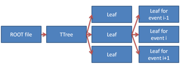
The hierarchy for the files are shown in the image below:

In Gate, the TTree is called Hits, and the leaves are named after the different variables that are automatically scored:

  PDGEncoding      - The Particle ID
  trackID          - Track number following a mother particle
  parentID         - The parent track's event ID. 0 if the current particle is a beam particle
  time             - Time in simulation (for ToF in PET, etc.)
  edep             - Deposited energy in this event / interaction
  stepLength       - The length of the current step
  posX             - Global X position of event
  posY             - Global Y position of event
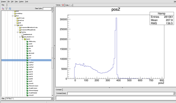
  posZ             - Global Z position of event
  localPosX        - Local (in mother volume) X position of event
  localPosY        - Local (in mother volume) Y position of event
  localPosZ        - Local (in mother volume) Z position of event
  baseID           - ID of mother volume scanner, == 0 if only one scanner defined
  level1ID         - ID of 1st level of volume hierarchy
  level2ID         - ID of 2nd level of volume hierarchy
  level3ID         - ID of 3rd level of volume hierarchy
  level4ID         - ID of 4th level of volume hierarchy
  sourcePosX       - Global X position of source particle
  sourcePosY       - Global Y position of source particle
  sourcePosZ       - Global X position of source particle
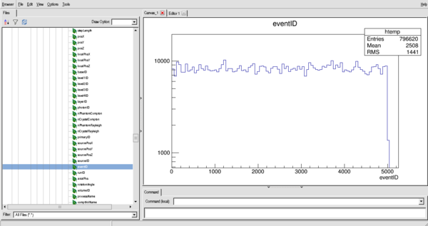
  eventID          - History number (important!!)
  volumeID         - ID of current volume (useful to isolate particles in a specific part of a fully scored volume)
  processName      - A string containing the name of the interaction type:
     - hIoni: Ionization by hadron
     - Transportation: No special interactions (usually from step limiter)
     - eIoni: Ionization by electron
     - ProtonInelastic: Inelastic nuclear interaction of proton
     - compt: Compton scattering
     - ionIoni: Ionization by ion
     - msc: Multiple Coulomb Scattering process
     - hadElastic: Elastic hadron / proton scattering

An example of the distribution of eventID (in histogram form, this is the number of interactions per particle (if bin size = 1))

  $ root
  ROOT [0] new TBrowser

Or for the Z distribution (see the Bragg Peak)

Opening the files in C++

It is quite simple to open the generated ROOT files in a C++ program.

In openROOTFile.C:

  #include <TTree.h>
  #include <TFile.h>
  
  using namespace std;
  
  void Run() {
     TFile *f = new TFile("gate_simulation.root");
     TTree *tree = (TTree*) f->Get("Hits"); // The TTree in the GATE file is called Hits
     
     // Declare the variables (leafs) to be readout
     Float_t x,y,z,edep;
     Int_t eventID, parentID;
     
     // Make a connection between the declared variables and the leafs
     tree->SetBranchAddress("posX", &x);
     tree->SetBranchAddress("posY", &y);
     tree->SetBranchAddress("posZ", &z);
     tree->SetBranchAddress("edep", &edep);
     tree->SetBranchAddress("eventID", &eventID);
     tree->SetBranchAddress("parentID", &parentID);
     
     // Loop over all the entries in the tree
     for (Int_t i=0, i < tree->GetEntries(); ++i) {
        tree->GetEntry(i);
        if (eventID > 2) break; // To limit the output!
        if (parentID != 0) continue; // Only show results from primary particles
  
        printf("Primary particle with event ID %d has an interaction with %.2f MeV energy loss at (x,y,z) = (%.2f, %.2f, %.2f).\n", eventID, edep, x, y, z);
     }
  
     delete f;
     }

Then you can run the program with

  $ root
  ROOT [0] .L openROOTFile.C+ // The + tells ROOT to compile the code
  ROOT [1] Run();

Please note that it is also possible to make a complete class to read out the root files using ROOT's MakeClass function. See [[3]].

Test case: Finding the range and straggling of a proton beam

  #include <TTree.h>
  #include <TH1F.h>
  #include <TFile.h>
  #include <TF1.h>
  
  using namespace std;
  
  void Run() {
     TFile  * f = new TFile("gate_simulation.root");
     TTree  * tree = (TTree*) f->Get("Hits"); // The TTree in the GATE file is called Hits
     TH1F   * rangeHistogram = new TH1F("rangeHistogram", "Stopping position for protons"; 800, 0, 400); // Histogram 1D with Float values
  
     Float_t  z;
     Int_t    eventID, parentID;
  
     Int_t    lastEventID = -1;
     Float_t  lastZ = -1;
     
     tree->SetBranchAddress("posZ", &z);
     tree->SetBranchAddress("eventID", &eventID);
     tree->SetBranchAddress("parentID", &parentID);
     
     for (Int_t i=0, i < tree->GetEntries(); ++i) {
        tree->GetEntry(i);
        if (parentID != 0) continue;
        
        // Check if this is the first event of a primary particle
        if (eventID != lastEventID && lastEventID >= 0) {
           rangeHistogram->Fill(lastZ);
        }
  
        // Store the current variables
        lastZ = z;
        lastEventID = eventID;
     }
  
     rangeHistogram->Draw();
   
     // Make a Gaussian fit to the range
     TF1 * fit = new TF1("fit", "gaus");
     rangeHistogram->Fit("fit", "", "", 150, 250); // Most probable values for fit is in this range, ROOT is quite sensitive to Gaussians occupying only a small part of the histogram, so give narrow fit range
  
     printf("The range of the proton beam is %.3f +- %.3f mm.\n", fit->GetParameter(1), fit->GetParameter(2));  
  }

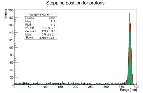
This time, the program will yield the following output (from a 250 MeV beam):

  The range of the proton beam is 378.225 mm +- 3.791 mm

With the following histogram (I've added some color and a SetOptFit to the legend)

Review of the analysis code by Helge Pettersen

Overview:

• Generating the GATE simulation files
• Perfoming GATE simulations
• Interlude - Tuning the analysis for the wanted geometry.
  • Making range-energy tables, finding the straggling, etc.
• Tracking analysis: This can be done both simplified and full
  • Simplified: No double-modelling of the pixel diffusion process (use MC provded energy loss), no track reconstruction (use eventID tag to connect tracks from same primary).
• The 3D reconstruction of phantoms using tracker planes has not yet been implemented
• Range estimation

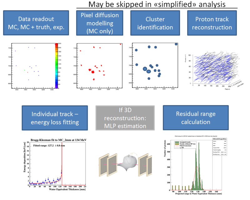
The analysis toolchain has the following components:

The full tracking workflow is implemented in the function DTCToolkit/HelperFunctions/getTracks.C::getTracks(), and the tracking and range estimation workflow is found in DTCToolkit/Analysis/Analysis.C::drawBraggPeakGraphFit().

GATE simulations

Geometry scheme

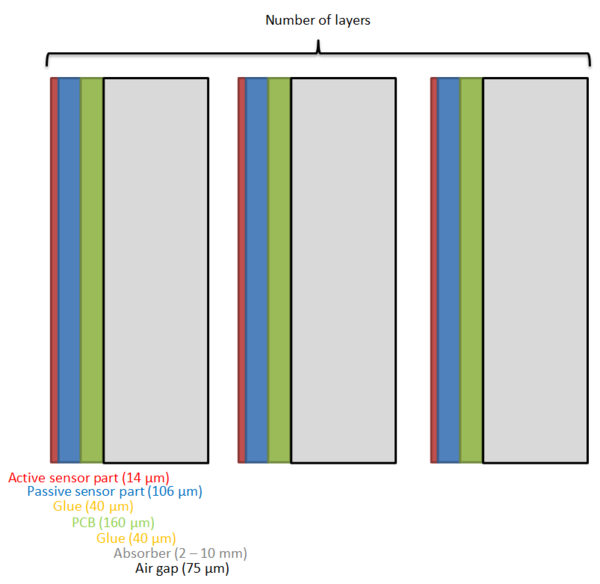
The simplified simulation geometry for the future DTC simulations has been proposed as:

It is partly based on the ALPIDE design, and the FoCal design. The GATE geometry corresponding to this scheme is based on the following hierarchy:

  World -> Scanner1 -> Layer -> Module + Absorber + Air gap
                                Module = Active sensor + Passive sensor + Glue + PCB + Glue
        -> Scanner2 -> [Layer] * Number Of Layers

The idea is that Scanner1 represents the first layer (where e.g. there is no absorber, only air), and that Scanner2 represents all the following (similar) layers which are repeated.

Generating the macro files

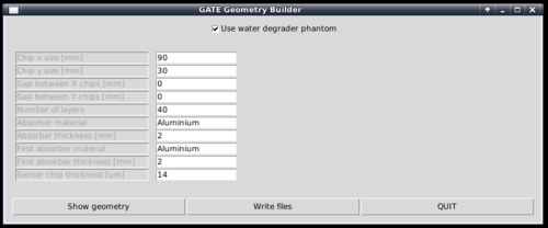
To generate the geometry files to run in Gate, a Python script is supplied. It is located within the gate/python subfolder.

   [gate/python] $ python gate/python/makeGeometryDTC.py

Choose the wanted characteristics of the detector, and use write files in order to create the geometry file Module.mac, which is automatically included in Main.mac. Note that the option "Use water degrader phantom" should be checked (as is the default behavior)!

Creating the full simulations files for a range-energy look-up-table

In this step, 5000-10000 particles are usually sufficient in order to get accurate results. To loop through different energy degrader thicknesses, run the script runDegraderFull.sh:

   [gate/python] $ sh runDegraderFull.sh <absorber thickness> <degraderthickness from> <degraderthickness stepsize> <degraderthickness to>

The brackets indicate the folder in the Github repository to run the code from.

For example, with a 3 mm degrader, and simulating a 250 MeV beam passing through a phantom of 50, 55, 60, 65 and 70 mm water:

   [gate/python] $ sh runDegraderFull.sh 3 50 5 70

Please note that there is a variable NCORES in this script, which ensures that NCORES versions of the Gate executable are run in parallel, and then waits for the last background process to complete before a new set of NCORES executables are run. So if you set NCORES=8, and run sh runDegraderFull.sh 3 50 1 70, first 50-57 will run in parallel, and when they're done, 58-65 will start, etc. The default value is NCORES=4.

Creating the chip-readout simulations files for resolution calculation

In this step a higher number of particles is desired. I usually use 25000 since we need O(100) simulations. A sub 1-mm step size will really tell us if we manage to detect such small changes in a beam energy.

And loop through the different absorber thicknesses:

   [gate/python] $ sh runDegrader.sh <absorber thickness> <degraderthickness from> <degraderthickness stepsize> <degraderthickness to>

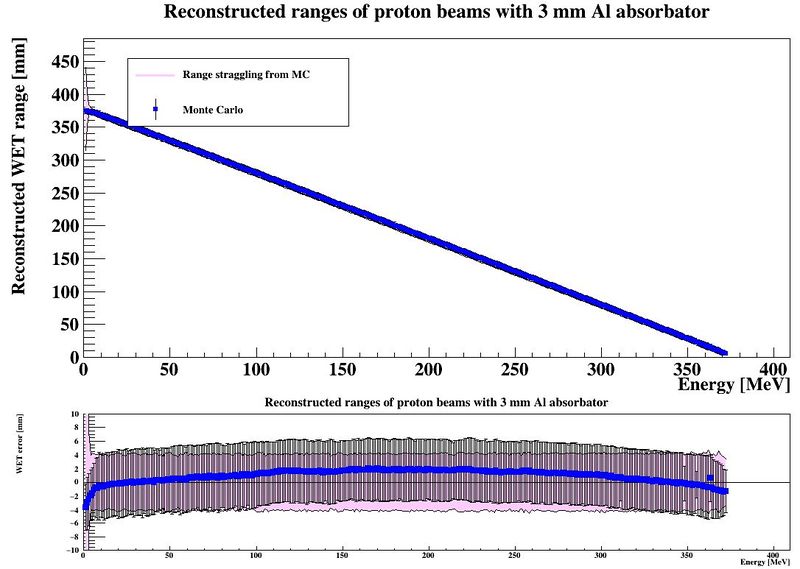
Creating the basis for range-energy calculations

The range-energy look-up-table

Now we have ROOT output files from Gate, all degraded differently through a varying water phantom and therefore stopping at different places in the DTC. We want to follow all the tracks to see where they end, and make a histogram over their stopping positions. This is of course performed from a looped script, but to give a small recipe:

1. Retrieve the first interaction of the first particle. Note its event ID (history number) and edep (energy loss for that particular interaction)
2. Repeat until the particle is outside the phantom. This can be found from the volume ID or the z position (the first interaction with {math|z>0}). Sum all the found edep values, and this is the energy loss inside the phantom. Now we have the "initial" energy of the proton before it hits the DTC
3. Follow the particle, noting its z position. When the event ID changes, the next particle is followed, and save the last z position of where the proton stopped in a histogram
4. Do a Gaussian fit of the histogram after all the particles have been followed. The mean value is the range of the beam with that particular "initial" energy. The spread is the range straggling. Note that the range straggling is more or less constant, but the contributions to the range straggling from the phantom and DTC, respectively, are varying linearly.

This recipe has been implemented in DTCToolkit/Scripts/findRange.C. Test run the code on a few of the cases (smallest and biggest phantom size ++) to see that

1. The correct start- and end points of the histogram looks sane. If not, this can be corrected for by looking how xfrom and xto is calculated and playing with the calculation.
2. The mean value and straggling is calculated correctly
3. The energy loss is calculated correctly

You can run findRange.C in root by compiling and giving it three arguments; Energy of the protons, absorber thickness, and the degrader thickness you wish to inspect.

   [DTCToolkit/Scripts] $ root 
   ROOT [1] .L findRange.C+
   // void findRange(Int_t energy, Int_t absorberThickness, Int_t degraderThickness)
   ROOT [2] findRange f(250, 3, 50); f.Run();

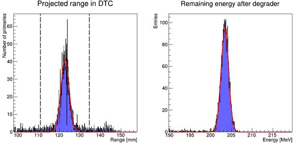
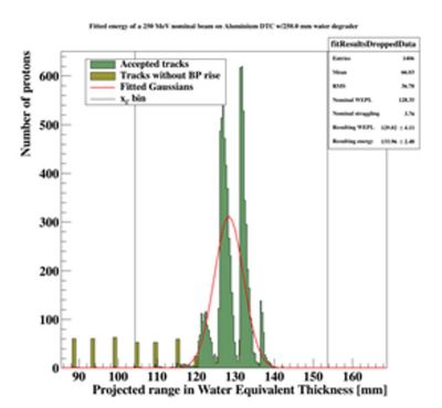
The output should look like this: Correctly places Gaussian fits is a good sign.

If you're happy with this, then a new script will run findRange.C on all the different ROOT files generated earlier.

   [DTCToolkit/Scripts] $ root 
   ROOT [1] .L findManyRangesDegrader.C
   // void findManyRanges(Int_t degraderFrom, Int_t degraderIncrement, Int_t degraderTo, Int_t absorberThicknessMm)
   ROOT [2] findManyRanges(50, 5, 70, 3)

This is a serial process, so don't worry about your CPU. The output is stored in DTCToolkit/Output/findManyRangesDegrader.csv. It is a good idea to look through this file, to check that the values are not very jumpy (Gaussian fits gone wrong).

We need the initial energy and range in ascending order. The findManyRangesDegrader.csv files contains more rows such as initial energy straggling and range straggling for other calcualations. This is sadly a bit tricky, but do (assuming a 3 mm absorber geometry):

  [DTCToolkit] $ cat OutputFiles/findManyRangesDegrader.csv | awk '{print ($6 " " $3)}' | sort -n > Data/Ranges/3mm_Al.csv

NB: If there are many different absorber geometries in findManyRangesDegrader, either copy the interesting ones or use | grep " X " | to only keep X mm geometry

When this is performed, the range-energy table for that particular geometry has been created, and is ready to use in the analysis. Note that since the calculation is based on cubic spline interpolations, it cannot extrapolate -- so have a larger span in the full Monte Carlo simulation data than with the chip readout. For more information about that process, see this document: File:Comparison of different calculation methods of proton ranges.pdf

Range straggling parameterization and [math]\displaystyle{ R_0 = \alpha E^p }[/math]

It is important to know the amount of range straggling in the detector, and the amount of energy straggling after the degrader. In addition, to calculate the parameters [math]\displaystyle{ \alpha, p }[/math] from the somewhat inaccurate Bragg-Kleeman equation [math]\displaystyle{ R_0 = \alpha E ^ p }[/math], in order to correctly model the "depth-dose curve" [math]\displaystyle{ dE / dz = p^{-1} \alpha^{-1/p} (R_0 - z)^{1/p-1} }[/math]. This is done by fitting the Bragg-Kleeman equation to the range-energy look up tables found by using DTCToolkit/Scripts/findManyRangesDegrader.C.

To find all this, run the script DTCToolkit/Scripts/findAPAndStraggling.C. This script will loop through all available data lines in the DTCToolkit/OutputFiles/findManyRangesDegrader.csv file that has the correct absorber thickness, so you need to clean the file first (or just delete it before running findManyRangesDegrader.C).

  [DTCToolkit/Scripts] $ root
  ROOT [0] .L findAPAndStraggling.C+
  // void findAPAndStraggling(int absorberthickness)
  ROOT [1] findAPAndStraggling(3)

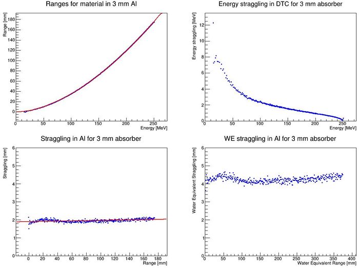
The output from this function should be something like this:

In addition, the following parameters should be extracted:

   Bragg-Kleeman parameters: R = 0.011626 E ^ 1.743151
   Straggling = 1.8568 + 0.000856 R

Configuring the DTC Toolkit to run with correct geometry

The values from findManyRanges.C should already be in DTCToolkit/Data/Ranges/3mm_Al.csv (or the corresponding material / thickness). Check that the file is correctly loaded in the file DTCToolkit/GlobalConstants/MaterialConstants.C. The values from findAPAndStraggling.C are put into the same file DTCToolkit/GlobalConstants/MaterialConstants.C:

   81  void createSplines() {
   ...   
   107    else if (kAbsorbatorThickness = 3) {
   108       in.open("Data/Ranges/3mm_Al.csv");
   109    }
   ...
   192    else if (kAbsorbatorThickness = 3) {
   193       alpha_aluminum = 0.011626;
   194       p_aluminum = 1.743151;
   195       straggling_a = 1.8568;
   196       straggling_b = 0.000856;
   197    }

Or in the corresponding material (alpha_pmma, alpha_carbon, etc.) and absorbatorthickness lines.

And in the file DTCToolkit/Scripts/makePlots.C, put the \alpha, p parameters.

   144   else if (absorberThickness == 3) {
   145      a_dtc = 0.011626;
   146      p_dtc = 1.743151;
   147    }

Then, look in the file DTCToolkit/GlobalConstants/Constants.h and check that the correct absorber thickness values etc. are set:

  ...
  39 Bool_t useDegrader = true;
  ...
  52 const Float_t kAbsorberThickness = 3;
  ...
  59 Int_t kEventsPerRun = 100000;
  ...
  66 const Int_t kMaterial = kAluminum;

Since we don't use tracking but only MC truth in the optimization, the number kEventsPerRun ([math]\displaystyle{ n_p }[/math] in the NIMA article) should be higher than the number of primaries per energy.

Running the DTC Toolkit

As mentioned, the analysis toolchain has the following components:

The following section will detail how to perform these separate steps. A quick review of the classes available:

• Hit: A (int x,int y,int layer, float edep) object from a pixel hit. edep information only from MC
• Hits: A TClonesArray collection of Hit objects
• Cluster: A (float x, float y, int layer, float clustersize) object from a cluster of Hits The (x,y) position is the mean position of all involved hits.
• Clusters: A TClonesArray collection of Cluster objects.
• Track: A TClonesArray collection of Cluster objects... But only one per layer, and is connected through a physical proton track. Many helpful member functions to calculate track properties.
• Tracks: A TClonesArray collection of Track objects.
• Layer: The contents of a single detector layer. Is stored as a TH2F histogram, and has a Layer::findHits function to find hits, as well as the cluster diffusion model Layer::diffuseLayer. It is controlled from a CalorimeterFrame object.
• CalorimeterFrame: The collection of all Layers in the detector.
• DataInterface: The class to talk to DTC data, either through semi-Hit objects as retrieved from Utrecht from the Groningen beam test, or from ROOT files as generated in Gate.

Important: To load all the required files / your own code, include your C++ sources files in the DTCToolkit/Load.C file, after Analysis.C has loaded:

  ...
  gROOT->LoadMacro("Analysis/Analysis.C+");
  gROOT->LoadMacro("Analysis/YourFile.C+"); // Remember to add a + to compile your code
  }

Data readout: MC, MC + truth, experimental

In the class DataInterface there are several functions to read data in ROOT format.

  int   getMCFrame(int runNumber, CalorimeterFrame *calorimeterFrameToFill, [..]) <- MC to 2D hit histograms
  void  getMCClusters(int runNumber, Clusters *clustersToFill); <-- MC directly to clusters w/edep and eventID
  void  getDataFrame(int runNumber, CalorimeterFrame *calorimeterFrameToFill, int energy); <- experimental data to 2D hit histograms

To e.g. obtain the experimental data, use

  DataInterface *di = new DataInterface();
  CalorimeterFrame *cf = new CalorimeterFrame();
  
  for (int i=0; i<numberOfRuns; i++) { // One run is "readout + track reconstruction
     di->getDataFrame(i, cf, energy);
     // From here the object cf will contain one 2D hit histogram for each of the layers
     // The number of events to readout in one run: kEventsPerRun (in GlobalConstants/Constants.h)
  }

Examples of the usage of these functions are located in DTCToolkit/HelperFunctions/getTracks.C. Please note the phenomenological difference between experimental data and MC:

• Exp. data has some noise, represented as "hot" pixels and 1-pixel clusters
• Exp. data has diffused, spread-out, clusters from physics processes
• Monte Carlo data has no such noise, and proton hits are represented as 1-pixel clusters (with edep information)

Pixel diffusion modelling (MC only)

To model the pixel diffusion process, i.e. the the diffusion of the electron-hole pair charges generated from the proton track towards nearby pixels, an empirical model has been implemented. It is described in the NIMA article [[4]], and also in the source code in DTCToolkit/Classes/Layer/Layer.C::diffuseLayer.

To perform this operation on a filled CalorimeterFrame *cf, use

  TRandom3 *gRandom = new TRandom3(0); // use #import <TRandom3.h>
  cf->diffuseFrame(gRandom);

Inverse pixel diffusion calculation (MC and exp. data)

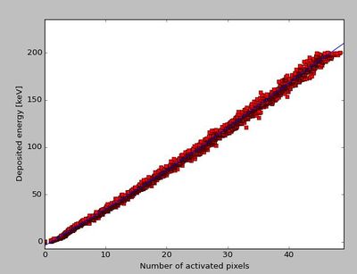
This process has been inversed in a Python script, and performed with a large number of input cluster sizes. The result is a parameterization between the proton's energy loss in a layer, and the number of activated pixels:

The function DTCToolkit/HelperFunctions/Tools.C::getEdepFromCS(n) contains the parameterization:

  Float_t getEdepFromCS(Int_t cs) {
     return -3.92 + 3.9 * cs - 0.0149 * pow(cs,2) + 0.00122 * pow(cs,3) - 1.4998e-5 * pow(cs,4);
  }

Cluster identification

Cluster identification is the process to find all connected hits (activated pixels) from a single proton in a single layer. It can be done by several algorithms, simple looped neighboring, DBSCAN, ... The process is such:

1. All hits are found from the diffused 2D histograms and stored as Hit objects with [math]\displaystyle{ (x,y,layer) }[/math] in a TClonesArray list.
2. This list is indexed by layer number (a new list with the index the first Hit in each layer) to optimize any search
3. The cluster finding algorithm is applied. For every Hit, the Hit list is looped through to find any connected hits. The search is optimized by use of another index list on the vertical position of the Hits. All connected hits (vertical, horizontal and diagonal) are collected in a single Cluster object with [math]\displaystyle{ (x,y,layer,cluster size) }[/math], where the cluster size is the number of its connected pixels.

This task is simply performed on a diffused CalorimeterFrame *cf:

  Hits *hits = cf->findHits();
  Clusters *clusters = hits->findClustersFromHits();

Proton track reconstruction

The process of track reconstruction is described fully in [[5]].

From a collection of cluster objects, Clusters * clusters, use the following code to get a collection of the Track objects connecting them across the layers.

  Tracks * tracks = clusters->findCalorimeterTracks();

Some optimization schemes can be applied to the tracks in order to increase their accuracy:

  tracks->extrapolateToLayer0(); // If a track was found starting from the second layer, we want to know the extrapolated vector in the first layer
  tracks->splitSharedClusters(); // If two tracks meet at the same position in a layer, and they share a single cluster, split the cluster into two and give each part to each of the tracks
  tracks->removeTracksLeavingDetector(); // If a track exits laterally from the detector before coming to a stop, remove it
  tracks->removeTracksEndingInBadChannnels(); // ONLY EXP DATA: Use a mask containing all the bad chips to see if a track ends in there. Remove it if it does.

Putting it all together so far

It is not easy to track a large number of proton histories simultaneously, so one may want to loop this analysis, appending the result (the tracks) to a larger Tracks list. This can be done with the code below:

  DataInterface *di = new DataInterface();
  CalorimeterFrame *cf = new CalorimeterFrame();
  Tracks * allTracks = new Tracks();
  
  for (int i=0; i<numberOfRuns; i++) { // One run is "readout + track reconstruction
     di->getDataFrame(i, cf, energy);
     TRandom3 *gRandom = new TRandom3(0); // use #import <TRandom3.h>
     cf->diffuseFrame(gRandom);
     Hits *hits = cf->findHits();
     Clusters *clusters = hits->findClustersFromHits();
     Tracks * tracks = clusters->findCalorimeterTracks();
     tracks->extrapolateToLayer0();
     tracks->splitSharedClusters();
     tracks->removeTracksLeavingDetector();
     tracks->removeTracksEndingInBadChannnels();
   
     for (int j=0; j<tracks->GetEntriesFast(); j++) {
        if (!tracks->At(j)) continue;
        allTracks->appendTrack(tracks->At(j));
     }
  
     delete tracks;
     delete hits;
     delete clusters;
  }

Individual tracks: Energy loss fitting

To obtain the most likely residual range / stopping range from a Track object, use

  track->doRangeFit();
  float residualRange = track->getFitParameterRange();

What happens here is that a TGraph with the ranges and in-layer energy losses of all the Cluster objects is constructed. A differentiated Bragg Curve is fitted to this TGraph:

[math]\displaystyle{ f(z) = p^{-1} \alpha^{-1/p} (R_0 - z)^{1/p-1} }[/math]

With [math]\displaystyle{ p,\alpha }[/math] being the parameters found during the full-scoring MC simulations. The value [math]\displaystyle{ R_0 }[/math], or track::getFitParameterRange is stored.

(3D reconstruction / MLP estimation)

When the volume reconstruction is implemented, it is to be put here:

1. Calculate the residual range and incoming vectors of all protons
2. Find the Most Likely Path (MLP) of each proton
3. Divide the proton's average energy loss along the MLP
4. Then, with a measure of a number of energy loss values in each voxel, perform some kind of average scheme to find the best value.

Instead, we now treat the complete detector as a single unit / voxel, and find the best SUM of all energy loss values (translated into range). The average scheme used in this case is described below, however this might be different than the best one for the above case.

Residual range calculation

To calculate the most likely residual range from a collection of individual residual ranges is not a simple task! It depends on the average scheme, the distance between the layers, the range straggling etc. Different solutions have been attempted:

• In cases where the distance between the layers is large compared to the straggling, a histogram bin sum based on the depth of the first layer identified as containing a certain number of proton track endpoints is used. It is the method detailed in the NIMA article [[6]], and it is implemented in DTCToolkit/Analysis/Analysis.C::doNGaussianFit(*histogram, *means, *sigmas).
• In cases where the distance between the layers is small compared to the straggling, a single Gaussian function is fitted on top of all the proton track endpoints, and the histogram bin sum average value is calculated from minus 4 sigma to plus 4 sigma. This code is located in DTCToolkit/Analysis/Analysis.C::doSimpleGaussianFit(*histogram, *means, *sigmas). This is the version used for the geometry optimization project.

With a histogram hRanges containing all the different proton track end points, use

  float means[10] = {};
  float sigmas[10] = {};
  TF1 *gaussFit = doSimpleGaussianFit(hRanges, means, sigmas);
  printf("The resulting range of the proton beam if %.2f +- %.2f mm.\n", means[9], sigmas[9]);

Geometry optimization: How does the DTC Toolkit calculate resolution?

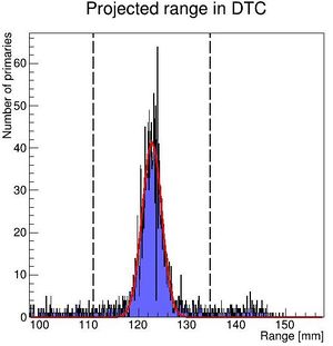
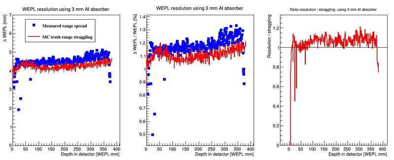
The resolution in this case is defined as the width of the final range histogram for all protons. The goal is to match the range straggling which manifests itself in the Gaussian distribution of the range of all protons in the DTC, from the full Monte Carlo simulations:

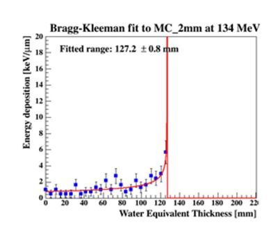
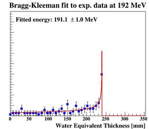
To characterize the resolution, a realistic analysis is performed. Instead of scoring the complete detector volume, including the massive energy absorbers, only the sensor chips placed at intervals ([math]\displaystyle{ \Delta z = 0.375\ \textrm{mm} + d_{\textrm{absorber}} }[/math]) are scored. Tracks are compiled by using the eventID tag from GATE, so that the track reconstruction efficiency is 100%. Each track is then put in a depth / edep graph, and a Bragg curve is fitted on the data:

The distribution of all fitted ranges (simple to calculate from fitted energy) should match the distribution above - with a perfect system. All degradations during analysis, sampling error, sparse sampling, mis-fitting etc. will ensure that the peak is broadened.

PS: Please forgive me the fact that the first figure is given in projected range, the second figure is given in initial energy and the third figure is given in projected water equivalent range...... They are converted losslessly since LUTs are used.

Finding the resolution

To find this resolution, or degradation in the straggling width, for a single energy, run the DTC toolkit analysis.

  [DTCToolkit] $ root Load.C
  // drawBraggPeakGraphFit(Int_t Runs, Int_t dataType = kMC, Bool_t recreate = 0, Float_t energy = 188, Float_t degraderThickness = 0)
  ROOT [0] drawBraggPeakGraphFit(1, 0, 1, 250, 34)

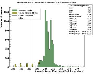
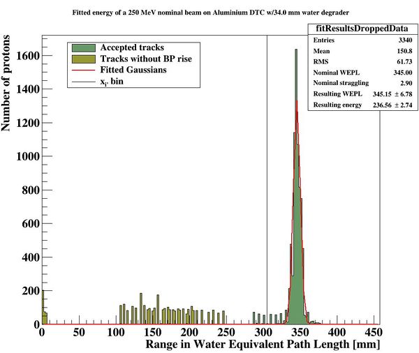
This is a serial process, so don't worry about your CPU when analysing all ROOT files in one go. With the result

The following parameters are then stored in DTCToolkit/OutputFiles/results_makebraggpeakfit.csv:

Absorber thickness	Degrader thickness	Nominal WEPL range	Calculated WEPL range	Nominal WEPL straggling	Calculated WEPL straggling
3 (mm)	34 (mm)	345 (mm WEPL)	345.382 (mm WEPL)	2.9 (mm WEPL)	6.78 (mm WEPL)

To perform the analysis on all different degrader thicknesses, use the script DTCToolkit/makeFitResultPlotsDegrader.sh (arguments: degrader from, degrader step and degrader to):

   [DTCToolkit] $ sh makeFitResultsPlotsDegrader.sh 1 1 380

This may take a few minutes... When it's finished, it's important to look through the file results_makebraggpeakfit.csv to identify all problem energies, as this is a more complicated analysis than the range finder above. If any is identified, run the drawBraggPeakGraphFit at that specific degrader thickness to see where the problems are.

Displaying the results

If there are no problems, use the script DTCToolkit/Scripts/makePlots.C to plot the contents of the file DTCToolkit/OutputFiles/results_makebraggpeakfit.csv:

  [DTCToolkit/Scripts/optimization] $ root plotRangesAndStraggling.C

The output is a map of the accuracy of the range determination, and a comparison between the range resolution (#sigma of the range determination) and its lower limit, the range straggling.

A review of the different modules in the code

The Digital Tracking Calorimeter Toolkit is located at Helge's github (but should be moved to the Gitlab when ready).

• https://github.com/HelgeEgil/focal

To clone the project, run

   git clone https://github.com/HelgeEgil/focal

in a new folder to contain the project. The folder structure will be

   DTCToolkit/                 <- the reconstruction and analysis code
   DTCToolkit/Analysis         <- User programs for running the code
   DTCToolkit/Classes          <- All the classes needed for the project
   DTCToolkit/Data             <- Data files: Range-energy look up tables, Monte Carlo code, LET data from experiments, the beam data from Groningen, ...
   DTCToolkit/GlobalConstants  <- Constants to adjust how the programs are run. Material parameters, geometry, ...
   DTCToolkit/HelperFunctions  <- Small programs to help running the code.
   DTCToolkit/OutputFiles      <- All output files (csv, jpg, ...) should be put here
   DTCToolkit/RootFiles        <- ROOT specific configuration files.
   DTCToolkit/Scripts          <- Independent scripts for helping the analysis. E.g. to create Range-energy look up tables from Monte Carlo data
   gate/                       <- All Gate-related files
   gate/python                 <- The DTC geometry builder
   projects/                   <- Other projects related to WP1

The best way to learn how to use the code is to look at the user programs, e.g. Analysis.C::DrawBraggPeakGraphFit which is the function used to create the Bragg Peak model fits and beam range estimation used in the 2017 NIMA article. From here it is possible to follow what the code does. It is also a good idea to read through what the different classes are and how they interact:

• Hit: A (int x,int y,int layer, float edep) object from a pixel hit. edep information only from MC
• Hits: A TClonesArray collection of Hit objects
• Cluster: A (float x, float y, int layer, float clustersize) object from a cluster of Hits The (x,y) position is the mean position of all involved hits.
• Clusters: A TClonesArray collection of Cluster objects.
• Track: A TClonesArray collection of Cluster objects... But only one per layer, and is connected through a physical proton track. Many helpful member functions to calculate track properties.
• Tracks: A TClonesArray collection of Track objects.
• Layer: The contents of a single detector layer. Is stored as a TH2F histogram, and has a Layer::findHits function to find hits, as well as the cluster diffusion model Layer::diffuseLayer. It is controlled from a CalorimeterFrame object.
• CalorimeterFrame: The collection of all Layers in the detector.
• DataInterface: The class to talk to DTC data, either through semi-Hit objects as retrieved from Utrecht from the Groningen beam test, or from ROOT files as generated in Gate.

To run the code, do

   [DTCToolkit] $ root Load.C

and ROOT will run the script Load.C which loads all code and starts the interpreter. From here it is possible to directly run scripts as defined in the Analysis.C file:

   ROOT [1] drawBraggPeakGraphFit(...)

DISCLAIMER: Some of the materials have been copied from the GATE v7.2 User's guide: http://wiki.opengatecollaboration.org/index.php/Users_Guide_V7.2

Troubleshooting

makeGeometryDTC.py - python ImportError: cannot import name _tkagg

The makeGeometryDTC.py scripts requires specific functionality in the python matplotlib. The following error can be solved by rebuilding matplotlib after installing the tk-dev package.

   Traceback (most recent call last):
     File "test.py", line 7, in <module>
       from matplotlib.backends.backend_tkagg import FigureCanvasTkAgg, NavigationToolbar2TkAgg
     File "/home/fieldsofgold/new/env/local/lib/python2.7/site-packages/matplotlib/backends/backend_tkagg.py", line 13, in <module>
       import matplotlib.backends.tkagg as tkagg
     File "/home/fieldsofgold/new/env/local/lib/python2.7/site-packages/matplotlib/backends/tkagg.py", line 7, in <module>
       from matplotlib.backends import _tkagg
   ImportError: cannot import name _tkagg

Rebuild matplotlib:

   sudo apt-get install tk-dev
   pip uninstall -y matplotlib
   pip --no-cache-dir install -U matplotlib